Empirical Analysis Applying Piecewise Constant Regression and Regression Splines
Introduction
In this assignment, I apply the method of piecewise constant regresion and regression splines to the export value with the fifth largest parteners reported by China from 1993 to 2017. The reason I exam this data set is that there are several exogenous strikes towards Chinese economy during this time period
- In 2001 China joined WTO.
- In 2008 financial crisis broke out.
Thus I expect the growth pattern before and after this two time cut will be different. I use R and imitate what Jiaming did to the wage data in the slides.
Code and Plotting
#Import the data and organize it to proper form
setwd("D:/All courses/Data Analysis for Economics(Microeconometrics)/HW2")
export<-read.csv("chnexport.csv")
library("tidyr")
export<-export[,-1]
export<-export[,-2:-5]
export<-export[order(export[,26],decreasing = TRUE),]
colnames(export)<-c("Name",1993:2017)
export<-export[1:15,]
ex<——gather(export,'1993','1994','1995','1996','1997','1998','1999','2000','2001','2002','2003','2004','2005','2006','2007','2008','2009','2010','2011','2012','2013','2014','2015','2016',key="Year",value="Export")
ex$Year<-as.numeric(ex$Year)
attach(ex)
Year.grid<-seq(1993,2017)
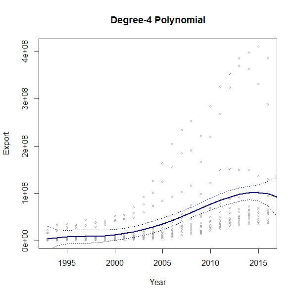
# Polynomial regression and plot
fit<-lm(Export~poly(Year,4))
pred<-predict(fit,newdata = list(Year=Year.grid),se=TRUE)
se.bands<-cbind(pred$fit+2*pred$se.fit,pred$fit-2*pred$se.fit)
plot(Year, Export, cex=.5, col="darkgrey")
lines(Year.grid, pred$fit, lwd=2, col="darkblue")
matlines(Year.grid, se.bands, lwd=1, col="darkblue", lty=3)
title("Degree-4 Polynomial")
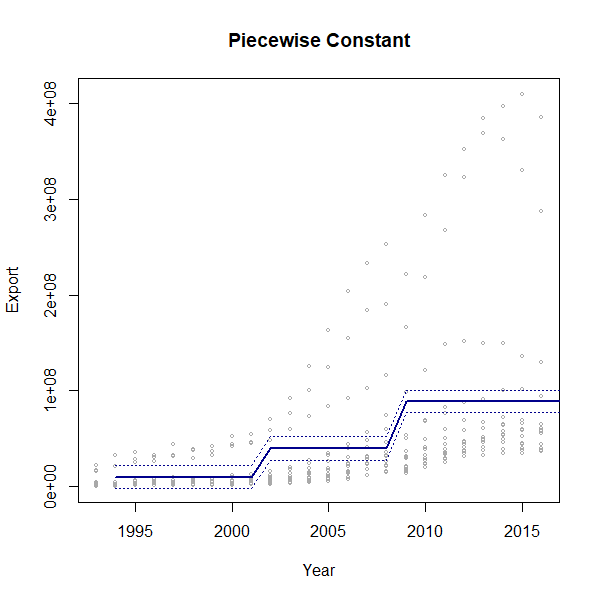
#Piecewise constant regression and plot
fitc<-lm(Export~0+cut(Year,c(1993,2001,2008,2017)))
predc<-predict(fitc,newdata = list(Year=Year.grid),se=TRUE)
se.bands.c<-cbind(predc$fit+2*predc$se.fit,predc$fit-2*predc$se.fit)
plot(Year,Export,cex=.5,col="darkgrey")
lines(Year.grid, predc$fit, lwd=2, col="darkblue")
matlines(Year.grid, se.bands.c, lwd=1, col="darkblue", lty=3)
title("Piecewise Constant")
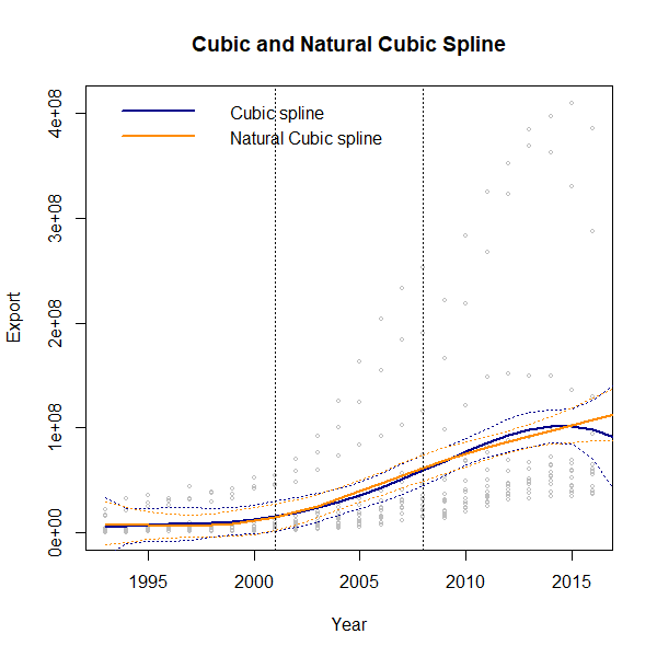
#Cubic spline and natural cubic spline and plot
fitbs<-lm(Export~bs(Year,knots = c(1993,2001,2008),degree=3))
predbs<-predict(fitbs,newdata = list(Year=Year.grid),se=TRUE)
se.bands.bs<-cbind(predbs$fit+2*predbs$se.fit,predbs$fit-2*predbs$se.fit)

fitns<-lm(Export~ns(Year,knots = c(1993,2001,2008)))
predns<-predict(fitns,newdata = list(Year=Year.grid),se=TRUE)
se.bands.ns<-cbind(predns$fit+2*predns$se.fit,predns$fit-2*predns$se.fit)

plot(Year,Export,cex=.5,col="grey")
lines(Year.grid,predbs$fit,lwd=2,col="darkblue")
matlines(Year.grid, se.bands.bs, lwd=1,col="darkblue",lty=3)
lines(Year.grid,predns$fit,lwd=2,col="darkorange")
matlines(Year.grid, se.bands.ns, lwd=1,col="darkorange",lty=3)
abline(v=c(2001,2008),lty=3)
legend("topleft",col=c("darkblue","darkorange"),lwd=2,legend = c("Cubic spline","Natural Cubic spline"),bty="n")
title("Cubic and Natural Cubic Spline")